
Implementation of breadth first search, depth first search and RRT
Grid search
Consider a 5 by 5 grid world. We would like to find a path from one end of the grid to the other end, that is from location (1,1) to location (5,5). The following algorithms are implemented to find this path:
1. Breadth first search
2. Depth first search
3. RRT
Optimality is defined as the least number of transitions required to reach the goal state.
Breadth first search
Breadth first search starts at the tree root and explores the neighbor nodes first, before moving to the next level neighbor nodes.
In this problem, since it is the number of transitions that we care about, once there is one path reaching the destination, all searches can stop.
Figure 1 shows the results generated by breadth first search. The vertical axis displays the discovering order of each node. For example, node (5,5) is the 25th node to be discovered. Therefore, its z-coordinate is 25. The optimal path takes 8 transitions from (1,1) to (5,5). All the nodes in the grid have been discovered. The number of times the search function was called was 23, since the search was terminated once the goal node was found.
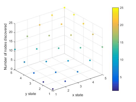
Figure 1. Breadth first search
Depth first search
Depth first search starts at the root and explores as far as possible along each branch before backtracking. Figure 2 shows the results generated by depth first search. The optimal path (there is only one path without backtracking) takes 24 transitions from (1,1) to (5,5). All the nodes in the grid have been discovered in just one shot (this is not common for depth first search without backtracking). The number of times the search function was called was 24. In this example, breadth first search seems to be superior to depth first search.
Depth first search starts at the root and explores as far as possible along each branch before backtracking. Figure 2 shows the results generated by depth first search. The optimal path (there is only one path without backtracking) takes 24 transitions from (1,1) to (5,5). All the nodes in the grid have been discovered in just one shot (this is not common for depth first search without backtracking). The number of times the search function was called was 24. In this example, breadth first search seems to be superior to depth first search.

Figure 2. Depth first search
RRT
An rapidly exploring random tree (RRT) grows a tree rooted at the starting configuration by using random samples from the search space. As each sample is drawn, a connection is attempted between it and the nearest state in the tree. If the connection is feasible (passes entirely through free space and obeys any constraints), this results in the addition of the new state to the tree. With uniform sampling of the search space, the probability of expanding an existing state is proportional to the size of its Voronoi region. As the largest Voronoi regions belong to the states on the frontier of the search, this means that the tree preferentially expands towards large unsearched areas.
Figure 3 shows the results generated by RRT. In this implementation, the random sample was uniformly distributed in the search space. It might be better if the sampling could be biased to those undiscovered area. The total number of samples and connection attempts was set to 100. In (a) and (c), the goal node was not reached in 100 attempts.
In run (b) and (d), 22 and 24 nodes in the grid were discovered, respectively. The optimal path takes 8 transitions from (1,1) to (5,5).


Figure 3. Rapid exploring random tree (4 runs)
|
|
| ||||||
