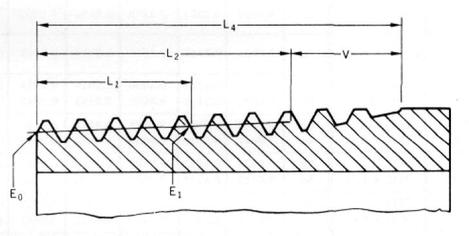
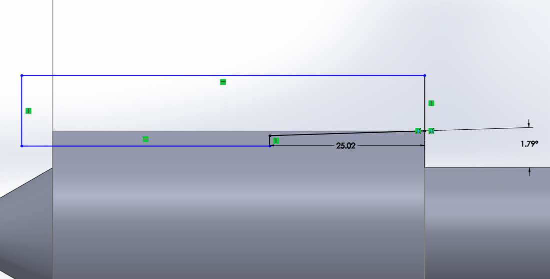
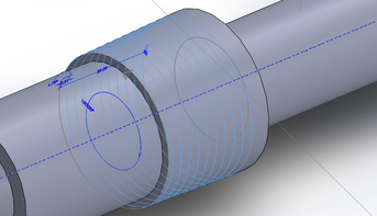
How to make nPT in Solidworks (American standard taper pipe threads size nPT chart attached)3/13/2015 National Pipe Thread Taper (NPT) is a U.S. standard for tapered threads used on threaded pipes and fittings. download:Make NPT in solidworks1. Determine the NPT thread size. 2. Find out the outside diameter of pipe according to the table. Draw a cylinder with that diameter. For example, for a NPT size of 1, the outside diameter of pipe is 1.315 inches = 33.4 mm. 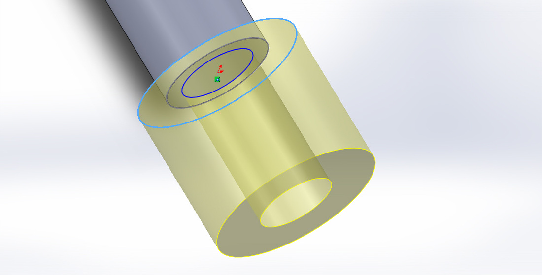 3. The taper rate for all NPT threads is 1 in 16 (3⁄4 inch per foot or 62.5 millimeters per meter) measured by the change of diameter (of the pipe thread) over distance. The angle between the taper and the center axis of the pipe is tan−1(1⁄32) = 1.7899° = 1° 47′ 24″. Be careful, it is not tan-1(1/16) here! Create the taper on the cylinder. 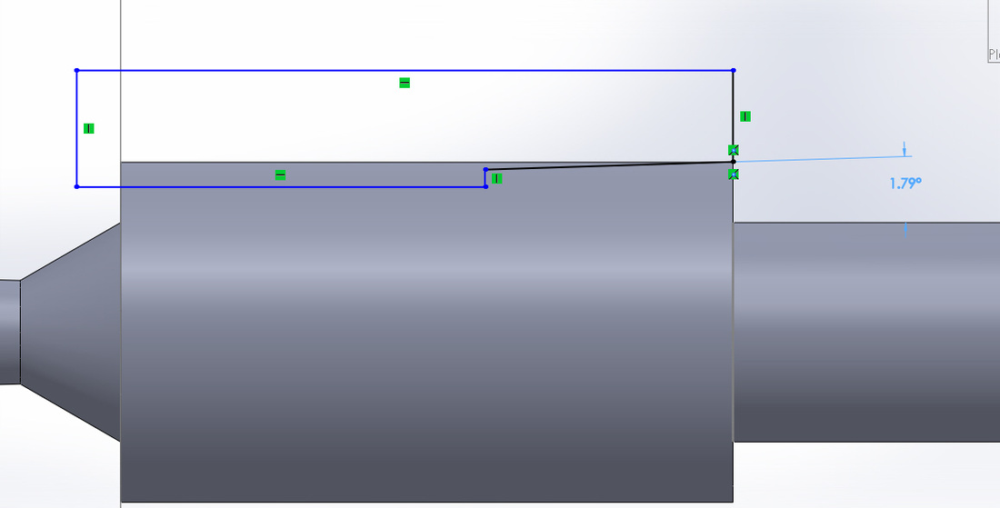 Revolved cut. 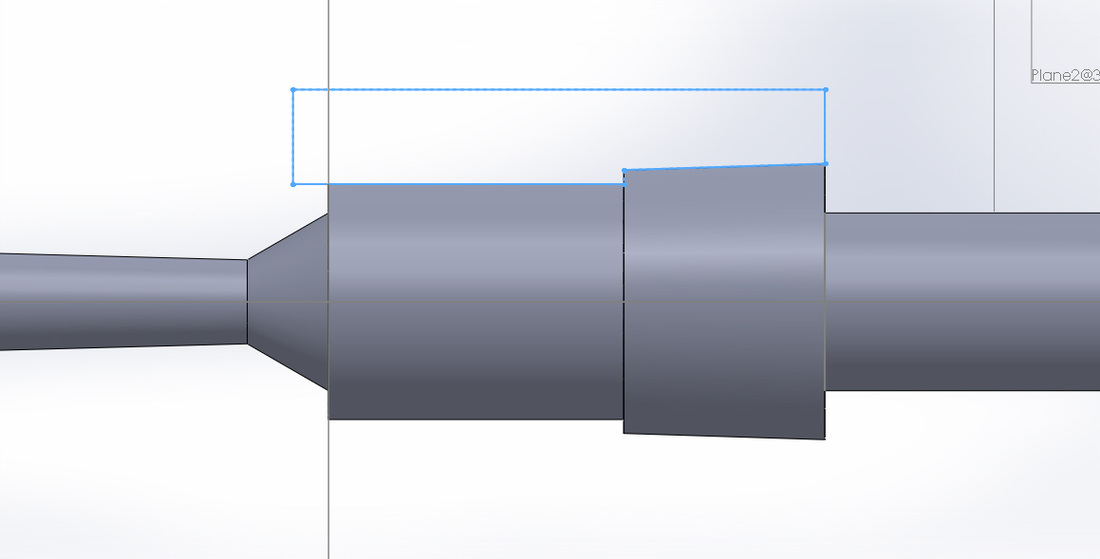 4. The basic effective length of the external taper thread, L2, includes two usable threads with slightly imperfect crests located against the the vanish threads. The length, L1, is the normal engagement between external and internal taper threads when screwed together hand tight. According to the table, for size 1, the effective thread length L2 should be 0.683 inches = 17.3482 mm and the vanish thread length V should be 0.302 inches = 7.6708 mm. Total length L4 = 0.985 inches = 25.02 mm.
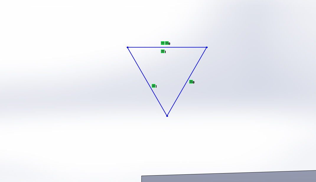
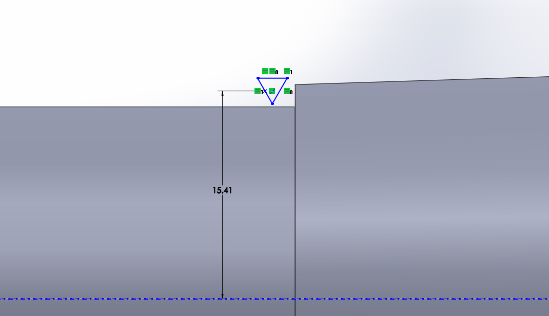
5. Create cutting profile. Draw a equilateral triangle. Find out the Pitch Diameter At Beginning of External Thread E0. This is the revolving diameter of the midpoint of the triangle at the beginning of the thread. Select the midpoint of one edge of the triangle. Set the distance between this point and the centerline according to E0. For NPT size of 1, E0 = 1.2136 inches = 30.825 mm.
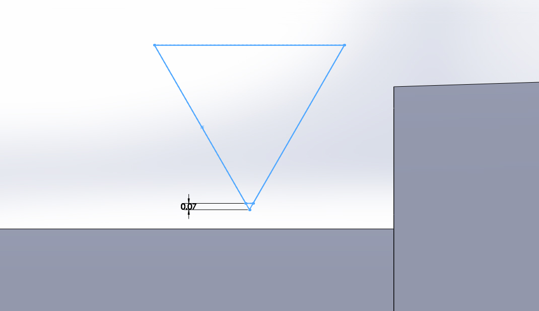
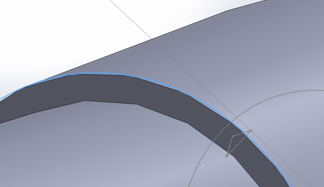
Instead of being a triangle, the cutter actually should look like which is highlighted with blue below. Its crest is truncated. Truncation crest or root for NPT 1 should be in the range of 0.0029 to 0.0063 inches (0.07366 mm to 0.16002 mm). The pitch of thread, which is the edge length of the triangle, should be 0.08696 inches = 2.209 mm.
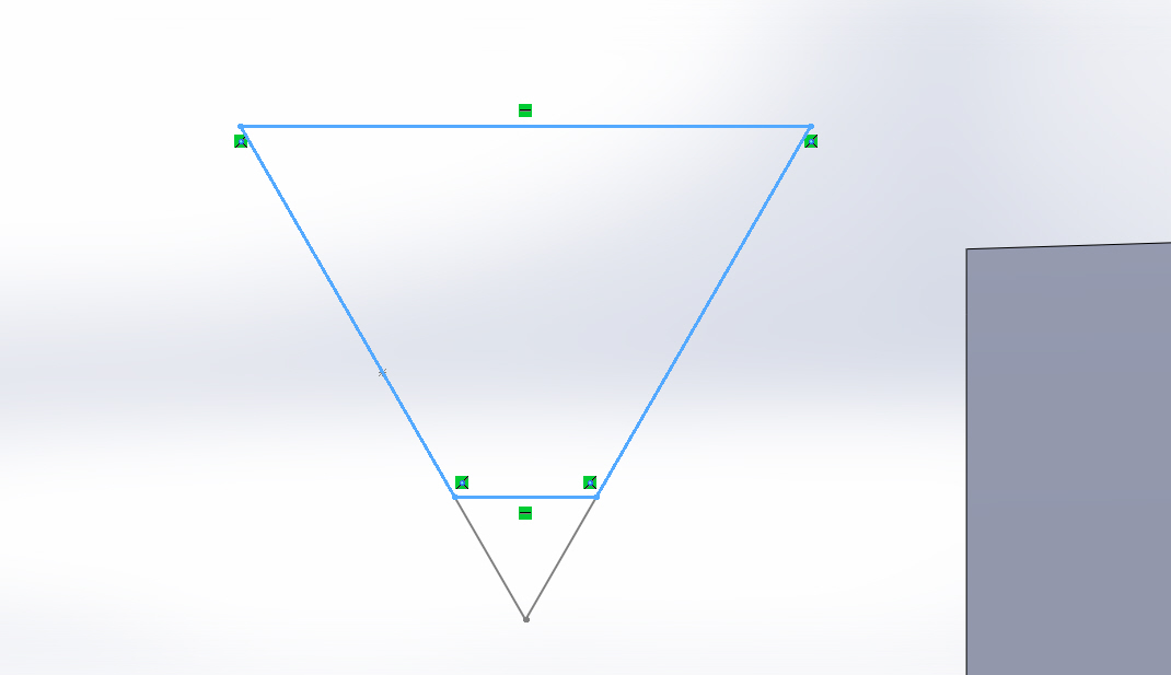
Shift the upper-right corner of the triangle to coincide with the beginning contour of the taper. 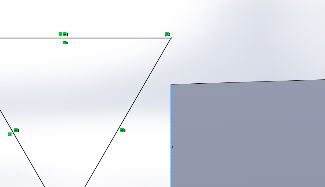 6. Create the helix contour to cut the threads, tapered outward 1.7899°. Sketch, convert the outline of the taper surface to sketch segment. Create the helix. Constant pitch equals 2.209 mm, clockwise, taper helix 1.7899° outward.
7. Sweep cut and create the thread. 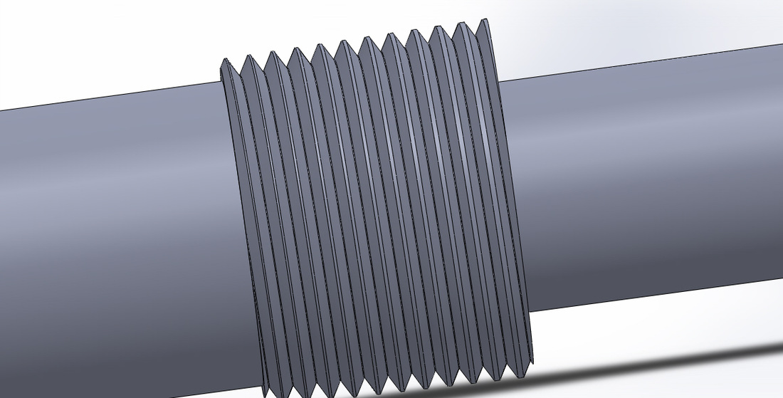 8. Further improvement. 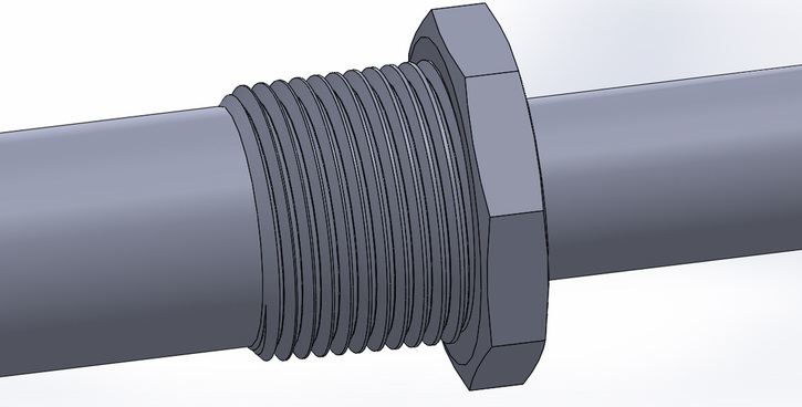 From THOMASNET.com Heat exchangers are devices whose primary responsibility is the transfer (exchange) of heat, typically from one fluid to another. However, they are not only used in heating applications, such as space heaters, but are also used in cooling applications, such as refrigerators and air conditioners. Many types of heat exchangers can be distinguished from on another based on the direction the liquids flow. In such applications, the heat exchangers can be and be parallel-flow, cross-flow, or counter-current. In parallel-flow heat exchangers, both fluid involved move in the same direction, entering and exiting the exchanger side by side. In cross-flow heat exchangers, the fluid paths run perpendicular to one another. In counter-current heat exchangers, the fluid paths flow in opposite directions, with each exiting where the other enters. Countercurrent heat exchangers tend to be more effective than other types of exchangers. Aside from classifying heat exchangers based on fluid direction, there are types that vary mainly in their composition. Some heat exchangers are comprised of multiple tubes, whereas others consist of hot plates with room for fluid to flow between them. It’s important to keep in mind that not all heat exchangers depend on the transfer of heat from liquid to liquid, but in certain cases use other mediums instead. Types of Heat Exchangers Shell and Tube Heat Exchanger Shell and tube heat exchangers are comprised of multiple tubes through which liquid flows. The tubes are divided into two sets: the first set contains the liquid to be heated or cooled. The second set contains the liquid responsible for triggering the heat exchange, and either removes heat from the first set of tubes by absorbing and transmitting heat away—in essence, cooling the liquid—or warms the set by transmitting its own heat to the liquid inside. When designing this type of exchanger, care must be taken in determining the correct tube wall thickness as well as tube diameter, to allow optimum heat exchange. In terms of flow, shell and tube heat exchangers can assume any of three flow path patterns. Plate Heat Exchanger Plate heat exchangers consist of thin plates joined together, with a small amount of space between each plate, typically maintained by a small rubber gasket. The surface area is large, and the corners of each rectangular plate feature an opening through which fluid can flow between plates, extracting heat from the plates as it flows. The fluid channels themselves alternate hot and cold fluids, meaning that heat exchangers can effectively cool as well as heat fluid—they are often used in refrigeration applications. Because plate heat exchangers have such a large surface area, they are often more effective than shell and tube heat exchangers. Regenerative Heat Exchanger In a regenerative heat exchanger, the same fluid is passed along both sides of the exchanger, which can be either a plate heat exchanger or a shell and tube heat exchanger. Because the fluid can get very hot, the exiting fluid is used to warm the incoming fluid, maintaining a near constant temperature. A large amount of energy is saved in a regenerative heat exchanger because the process is cyclical, with almost all relative heat being transferred from the exiting fluid to the incoming fluid. To maintain a constant temperature, only a little extra energy is need to raise and lower the overall fluid temperature. Plate Fin Heat Exchanger A plate-fin heat exchanger is a type of heat exchanger design that uses plates and finned chambers to transfer heat between fluids. It is often categorized as a compact heat exchanger to emphasise its relatively high heat transfer surface area to volume ratio. The plate-fin heat exchanger is widely used in many industries, including the aerospace industry for its compact size and lightweight properties, as well as in cryogenics where its ability to facilitate heat transfer with small temperature differences is utilized. Aluminum alloy plate fin heat exchangers have been used in the aircraft industry for 50 years and in cryogenics and chemical plant for 35 years. They are also used in railway engines and motor cars. Stainless steel plate fins have been used in aircraft for 30 years and are now becoming established in chemical plant. Adiabatic Wheel Heat Exchanger In this type of heat exchanger, an intermediate fluid is used to store heat, which is then transferred to the opposite side of the exchanger unit. An adiabatic wheel consists of a large wheel with threads that rotate through the fluids-both hot and cold-to extract or transfer heat. Useful Links GEA Flat Plate Heat Exchanger Online Selection
Overview
The basic function provided by EES is the solution of a set of algebraic equations. EES can also solve differential equations, equations with complex variables, do optimization, provide linear and non-linear regression, generate publication-quality plots, simplify uncertainty analyses and provide animations. EES allows the user to enter his or her own functional relationships in three ways. First, a facility for entering and interpolating tabular data is provided so that tabular data can be directly used in the solution of the equation set. Second, the EES language supports user-written Functions and Procedures similar to those in Pascal and FORTRAN. EES also provides support for user-written routines, which are self-contained EES programs that can be accessed by other EES programs. The Functions, Procedures, Subprograms and Modules can be saved as library files which are automatically read in when EES is started. Third, external functions and procedures, written in a high-level language such as Pascal, C or FORTRAN, can be dynamically-linked into EES using the dynamic link library capability incorporated into the Windows operating system. These three methods of adding functional relationships provide very powerful means of extending the capabilities of EES. Interesting practical problems that may have implicit solutions, such as those involving both thermodynamic and heat transfer considerations, are often not assigned because of their mathematical complexity. EES allows the user to concentrate more on design by freeing him or her from mundane chores. EES is particularly useful for design problems in which the effects of one or more parameters need to be determined. A new user should read Chapter 1 which illustrates the solution of a simple problem from start to finish. Chapter 2 provides specific information on the various functions and controls in each of the EES windows. The animation capabilities provided in the Diagram window are described in this chapter. Chapter 3 is a reference section that provides detailed information for each menu command. Chapter 4 describes the built-in mathematical and thermophysical property functions and the use of the Lookup Table for entering tabular data. Chapter 5 provides instructions for writing EES Functions, Procedures, Subprograms and Modules and saving them in Library files. Chapter 6 describes how external functions and procedures, written as Windows dynamic-link library (DLL) routines, can be integrated with EES. Chapter 7 describes a number of advanced features in EES such as the use of string, complex and array variables, the solution of simultaneous differential and algebraic equations, and property plots. The use of directives and macros is also explained. Appendix A contains a short list of suggestions. Appendix B describes the numerical methods used by EES. Appendix C shows how additional property data may be incorporated into EES.
Inside a kettle (Hele-Shaw cell heated from below) Hele-Shaw cell: A Hele-Shaw cell consists of two flat plates that are parallel to each other and separated by a small distance. At least one of the plates is transparent. These cells are used for studying many phenomena, including the behavior of granular materials as they are being poured into the space between the plates. A more complete technical name is a quasi-two-dimensional Hele-Shaw cell. "This fluid dynamics video images the different heat transport mechanisms at play when a liquid confined in a vertical Hele-Shaw cell is heated from below. The two-dimensional time resolved temperature field inside the cell is measured by a quantitative Schlieren technique which is detailed in the video." "When a liquid in a container is heated from below and cooled from the top a heat flux settles through the liquid. As the temperature of the bottom plate increases, the heat transport is successively dominated by different mechanisms: conduction, convection and boiling. To study this, experiments with a Hele-Shaw cell were undertaken. Instantaneous non-intrusive measurements of the two-dimensional temperature field are performed in the cell. The video presents these measurements in combination with Schlieren visualizations of the flow to illustrate the different heat transport mechanisms and the transitions between them. The cell is made of two thin vertical glass slides (50 mm in width and 25 mm in height) separated by a 1 mm gap. The bottom of the cell is made of a thin heat-conducting plate. The top is open. The movie begins when a cell filled with ethanol at ambient temperature is put on top of a hot copper block. In order to visualize the temperature evolution inside the cell a screen patterned with a regular cross-ruling is put behind the cell. As the liquid in the cell warms up, the cross-ruling, as seen through the cell, looks distorted. The temperature differences in the cell plane give rise to index of refraction gradients. This bends the light rays, resulting in a distorted image of the cross-ruling. Because the index of refraction-temperature relationship and the distance to the screen are known, measurements of the distortion can be used to calculate the temperature gradients in the cell. By integrating those gradients, this technique provides the temperature field inside the cell with a time resolution that is only limited by the camera frame rate (here 500 frames per second). This is used in the video to illustrate the different heat transport mechanisms at play as the liquid inside the cell is heated from below to progressively higher temperatures. One successively observes the temperature fields for: (1) two-dimensional convection motions with light, hot plumes rising between falling heavy, cold ones, (2) nucleate boiling of vapor bubbles on the bottom plate as the ethanol boiling temperature is exceeded, (3) and the `boiling crisis', i.e. the transition to the film boiling regime where the bottom plate is covered by a vapor film which periodically destabilizes by a Rayleigh-Taylor instability." Key points: The expansion through the nozzle is so quick that condensation within the vapor does not occur (due to very small time). The vapor expand as superheated vapor until some point at which condensation occurs suddenly and irreversibly. Heat And Mass Transfer With The volume of fluid Model And Evaporation-Condensation ModelTo be added. Heat and mass transfer with the mixture model and evaporation-condensation modelTo be added. videosHeat and mass transfer between two phases (half liquid) using the Volume of Fluid (VOF) multi-phase model in ANSYS FLUENT along with Evaporation-Condensation model - Contours of volume of fluid Heat and mass transfer with the mixture model and evaporation-condensation model - Contours of static temperature (mixture) Heat and mass transfer with the mixture model and evaporation-condensation model - Contours of velocity magnitude (mixture) referenceTutorial: Using the Volume of Fluid (VOF) model
Introduction to User Defined Functions (UDF)
Examples of User Defined Functions (UDF)
Fluent User Defined Functions (UDF) manual
Tutorial: comparison of using the mixture and eulerian multiphase models
Horizontal film boiling simulation by Fluent
Good video of CFD nucleate boiling using FLUENT / ANSYS by M. Habte. Ph.D., Mechanical Engineering CFD Simulation of Pool Boiling Phenonmena by Yi Liu. Different boiling phenonmena including Film boiling, Transition boiling and Nucleate boiling are identified by CFD simulation. |
Jingwei ZhuPh.D. candidate in the Department of Mechanical Science and Engineering at the University of Illinois at Urbana-Champaign. 
Categories
All
Archives
October 2018
|
||||||||||||||||||||||||

|
|
 RSS Feed
